In my previous post, I laid out the broad goal of this project: to assess the feasibility of reforestation and biodiversity support along the Interstate 90 corridor in the Washington Cascades—especially in areas where wildlife crossings or ecological restoration might enhance long-term habitat connectivity.
However, after publishing that update and revisiting my datasets, I realized that I had mistakenly labeled the study area as being along Interstate 90. In reality, the initial model I built was based on a mountainous stretch near U.S. Highway 2, which also traverses the Cascades and passes through Snoqualmie and Stevens Pass.
While this mistake doesn’t invalidate the raster modeling process I used, I’ve updated my map and post to reflect the correct highway and will use this moment as a learning opportunity in how cartographic missteps can happen when working with basemaps that lack clear road labels.
The Study Area (Revised)
The original model focused on a mountainous section of U.S. Highway 2 near Stevens Pass—a scenic but rugged corridor that, like I‑90, cuts through the Cascade Range and serves as a vital east-west link. This region is also ecologically important, with ongoing efforts to improve wildlife mobility and habitat health.
Method: A Simple Raster Overlay
To get the project started, I built a basic raster-based suitability model using two variables: land cover and terrain slope. This would provide a rough initial screen for areas where reforestation or habitat restoration might be viable.
1. Land Cover
I reclassified NLCD land cover classes into suitability scores as follows:
- 7 – Grassland/Herbaceous
- 5 – Shrub/Scrub
- 0 – All other classes (considered unsuitable for restoration without major intervention)
These categories were selected for their potential to support reforestation without significant clearing or conflict with existing development.
2. Slope
I derived a percent-slope raster from a digital elevation model (DEM) and reclassified it into:
- 9 – Gentle terrain (0–10%)
- 7 – Moderate (10–20%)
- 5 – Semi-steep (20–30%)
- 3 – Steep (30–40%)
- 1 – Very steep (40–60%)
- 0 – Unsuitable (>60%)
3. Raster Calculator
To combine these factors, I used the following weighted formula in Raster Calculator:
("Reclass_LandCover_Habitat" * 0.6) + ("Reclass_Slope_Habitat" * 0.4)
This produced a final suitability score between 1 and 10, with higher scores indicating better conditions for habitat restoration.
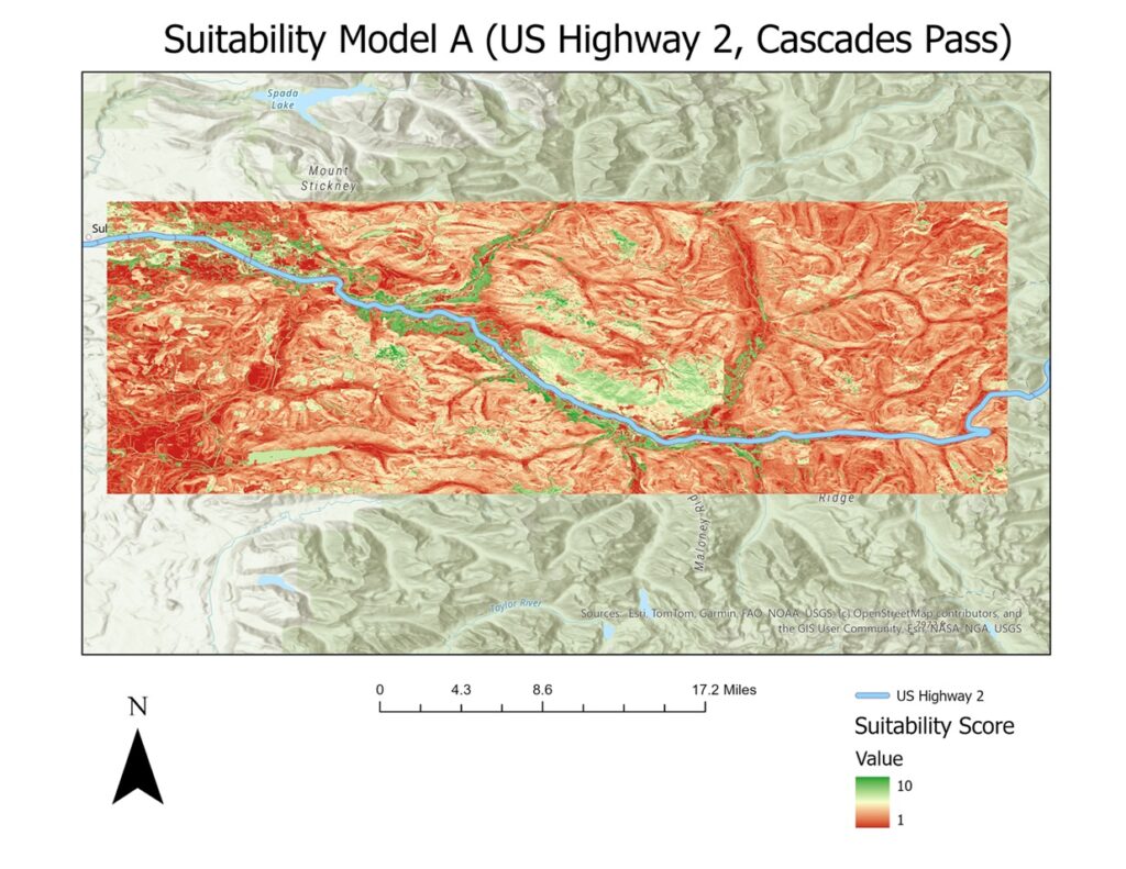
Results
Despite the steep terrain dominating the area near U.S. Highway 2, the model identified several promising pockets of higher suitability—often in valleys, foothills, and roadside clearings.
While this initial output isn’t comprehensive, it serves as a valuable first-pass screen for identifying potential opportunity zones.
Lessons Learned
This phase of the project underscored a simple but powerful lesson: when road labels are missing or unclear, even experienced GIS users can mix up key reference features. Fortunately, the modeling workflow itself remains valid and can easily be adjusted for additional locations—including Interstate 90, which I still intend to analyze in the next phase.